Section 0: Module Objectives or Competencies
| Course Objective or Competency | Module Objectives or Competency |
|---|---|
| The student will be able to list and explain basic data warehouse concepts. | The student will be able to explain the basic concepts of dimensional modeling, including dimension tables and fact tables. |
| The student will be able to explain the most commonly used data warehouse modeling strategies with respect to how they utilize ER modeling, relational modeling, and dimensional modeling. |
Section 1: Data Warehouse Modeling Approaches
Both ER modeling and relational modeling can be used in the development of data warehouses.
The following are three of the most common data warehouse and data mart modeling approaches:
- Normalized data warehouse
- Dimensionally modeled data warehouse
- Independent data marts
Section 2: Normalized Data Warehouse
Envisions a data warehouse as an integrated analytical database modeled by using traditional database modeling techniques like ER modeling and relational modeling, resulting in a normalized relational database schema.
- Populated with analytically useful data from the operational data sources via the ETL process.
- Serves as a source of data for dimensionally modeled data marts and for any other non-dimensional analytically useful data sets.
The following figure illustrates a normalized data warehouse.
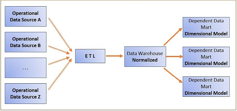
The idea behind this method is to have a central data warehouse modeled as an ER model that is subsequently mapped into a normalized relational database model.
- The normalized relational database serves as a physical store for the data warehouse.
- All integration of the underlying operational data sources occurs within a central normalized database schema.
- Once a data warehouse is completed and populated with the data from the underlying sources via the ETL infrastructure, various analytically useful views, subsets, and extracts are possible based on this fully integrated database.
- One of the primary types of analytical data sets resulting from the normalized data warehouse is a dimensionally modeled data mart, which can then be queried using OLAP/BI tools.
- Other, non-dimensional data sets can also be extracted when they are needed for analysis and decision support.
Section 3: Dimensionally Modeled Data Warehouse
Views a data warehouse as a dimensional model that integrates analytically useful information from the operational data sources.
The following figure illustrates a normalized data warehouse.
- While this approach is the same as the normalized data warehouse approach when it comes to the utilization of operational data sources and the ETL process, the difference is the technique used for modeling the data warehouse.
-
A set of commonly used dimensions known as conformed dimensions is designed first.
- Fact tables corresponding to the subjects of analysis are then subsequently added.
- For example, in a retail company, conformed dimensions such as CALENDAR, PRODUCT, and STORE can be designed first, as they will be commonly used by subjects of analysis.
- A set of dimensional models is created in which each fact table is connected to multiple dimensions, and some of the dimensions are shared by more than one fact table.
-
In addition to the originally created set of conformed dimensions, other dimensions are included as needed, resulting in a data warehouse that is a dimensional model with multiple fact tables.
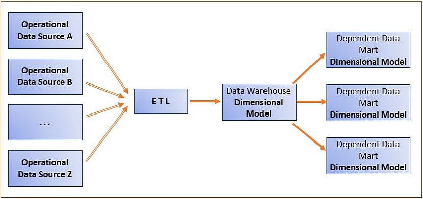
- The result is a data warehouse that is a dimensional model with multiple fact tables, i.e. a constellation of stars.
A dimensionally modeled data warehouse can be used as a source for dependent data marts and other views, subsets, and/or extracts.
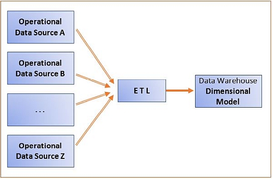
Section 4: Independent Data Marts
In this method, stand–alone data marts are created by various groups within the organization, independent of other stand–alone data marts in the organization, and as a consequence, multiple ETL systems are created and maintained.
-
Independent data marts are considered an inferior strategy.
- Inability for straightforward analysis across the enterprise.
- The existence of multiple unrelated ETL infrastructures.
- In spite of obvious disadvantages, a significant number of corporate analytical data warehouses are developed as a collection of independent data marts, often due to a lack of initial enterprise-wide focus when data analysis is addressed.
Section 5: Dimensional Modeling
Dimensional Modeling: Introduction (begin at the 4:10 mark)
Dimensional modeling, a modeling technique tailored specifically for subject-oriented analytical data warehouse and data mart design purposes, is the preferred technique for presenting analytic data.
- It stores data in such a way that it is relatively easy to retrieve the data once it is stored in database.
- To build a dimensional database, you start with a dimensional data model.
- The dimensional data model provides a method for making databases simple and understandable.
Before exploring dimensional modeling, we need to understand facts and dimensions. These are critical data warehousing concepts.
Facts
A fact is a quantitative piece of information.
-
Facts are stored in fact tables.
- Fact tables are the foundation of a dimensional data warehouse.
- Fact tables contain the measurement of factors that have some analytical value.
- Fact tables have a foreign key relationship with a number of dimension tables.
Dimensions
A dimension is a set of data attributes pertaining to something of interest to a business.
-
Dimensions are stored in dimension tables that contain attributes of measurements stored in fact tables.
- Dimensions can be anything which can consistently categorize data, and provide a analytically useful perspective
- Therefore, a dimension is a collection of reference information about facts.
- Dimensions categorize and describe data warehouse facts and measures in ways that support meaningful answers to analytical questions.
Fact Tables and Dimension Tables
A fact table holds the data to be analyzed, and a dimension table stores data about the ways in which the data in the fact table can be analyzed. Hence, fact tables have more records than dimension tables. fact table
In addition to using regular relational concepts (primary keys, foreign keys, integrity constraints, etc.) dimensional modeling distinguishes two types of tables:
-
Dimension tables
- Contain descriptions of the business, organization, or enterprise to which the subject of analysis belongs.
- Columns in dimension tables contain descriptive information that is often textual (e.g., product brand, product color, customer gender, customer education level), but can also be numeric (e.g., product weight, customer income level).
-
This information provides a basis for analysis of the subject.
- For example, if the subject of the business analysis is sales, it can be analyzed by product brand, customer gender, customer income level, and so on.
-
Fact tables
- Contain quantitative measures related to the subject of analysis.
- Also contain foreign keys that associate fact tables with dimension tables.
-
The measures in the fact tables are typically numeric and are intended for mathematical computation and quantitative analysis.
- For example, if the subject of the business analysis is sales, one of the measures in the fact table sales could be the sales dollar amount.
- The sale amounts can be calculated and recalculated using different mathematical functions across various dimension columns.
- By way of illustration, the total and average sale can be calculated per product brand, customer gender, customer income level, and so on.
Star schema
- The result of dimensional modeling is a dimensional schema containing facts and dimensions.
- The dimensional schema is often referred to as the star schema
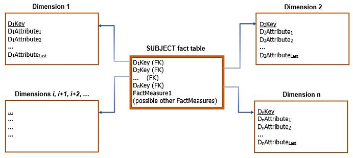
- A dimension table contains a primary key and attributes that are used for analysis of the measures in the fact tables.
-
A fact table contains fact-measure attributes and foreign keys that connect the fact table to the dimension tables.
- The primary key of a fact table is a composite key that combines foreign key columns and/or other columns in the fact table.
- Fact tables are indicated by a thicker frame to distinguish them from the dimension tables in the figures, and measures in the fact tables always appears as the last columns in the table.
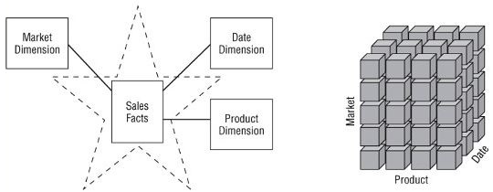
Dimensional Model (Star Schemas and OLAP Cubes)
You can conceive of a dimensional database as a database cube of three or four dimensions where users can access a slice of the database along any of its dimensions.
Both stars and cubes have a common logical design with recognizable dimensions; however, the physical implementation differs (see figure below).
A star schema can be physically implemented in the form of a cube.
OLAP Cubes
- Referred to as online analytical processing (OLAP) cubes in multidimensional database platforms.
- Cubes can deliver superior query performance because of the precalculations, indexing strategies, and other optimizations.
- See The Multidimensional Data Model and Multidimensional Data Modeling – OLAP Cubes for a more detailed discussion.
Section 6: Initial Example: Dimensional Model Based on A Single Source
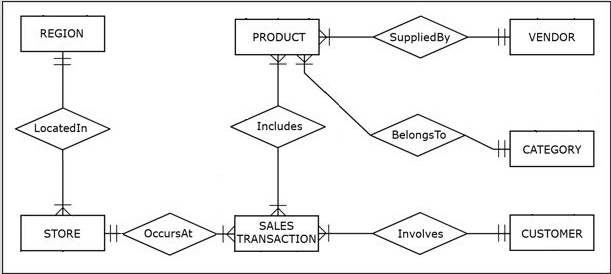
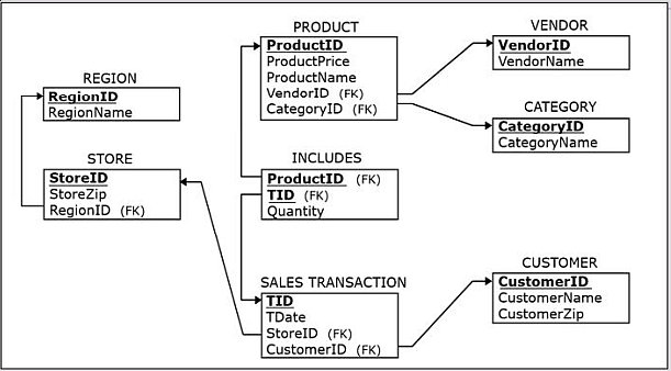
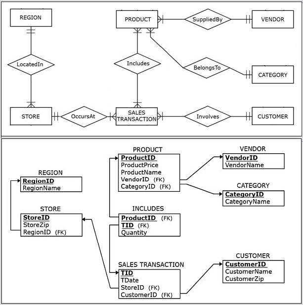
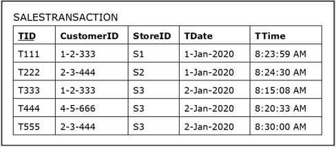
The following figures show the ER diagram and the resulting relational schema for a sales department database.
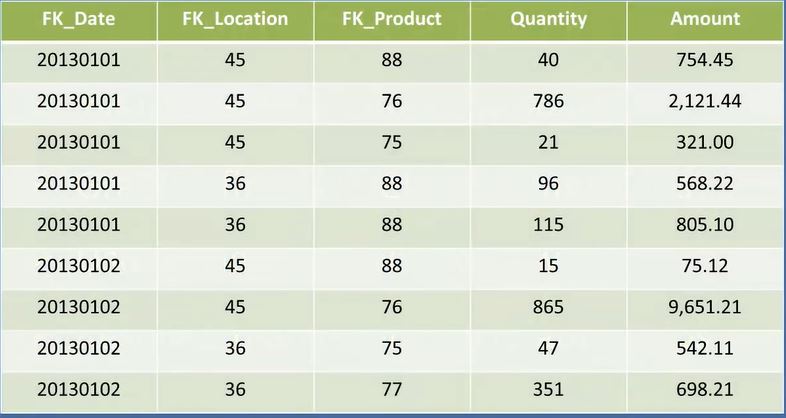
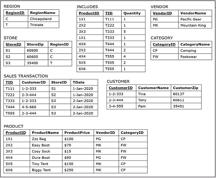
The following figure show data records for the sales department database.
Based on the operational database shown in the above figures, the dimensional modeling technique can be used to design an analytical database whose subject of analysis is sales.
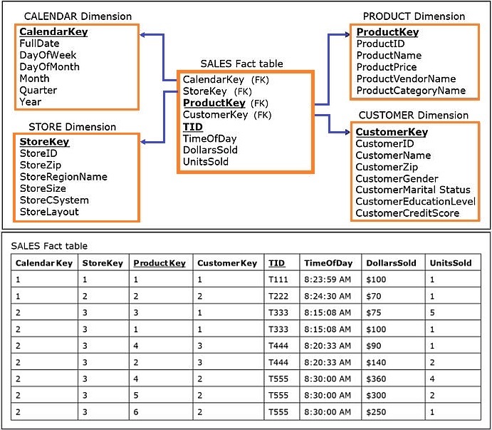
- The result of this process is the star schema shown in the figure below.
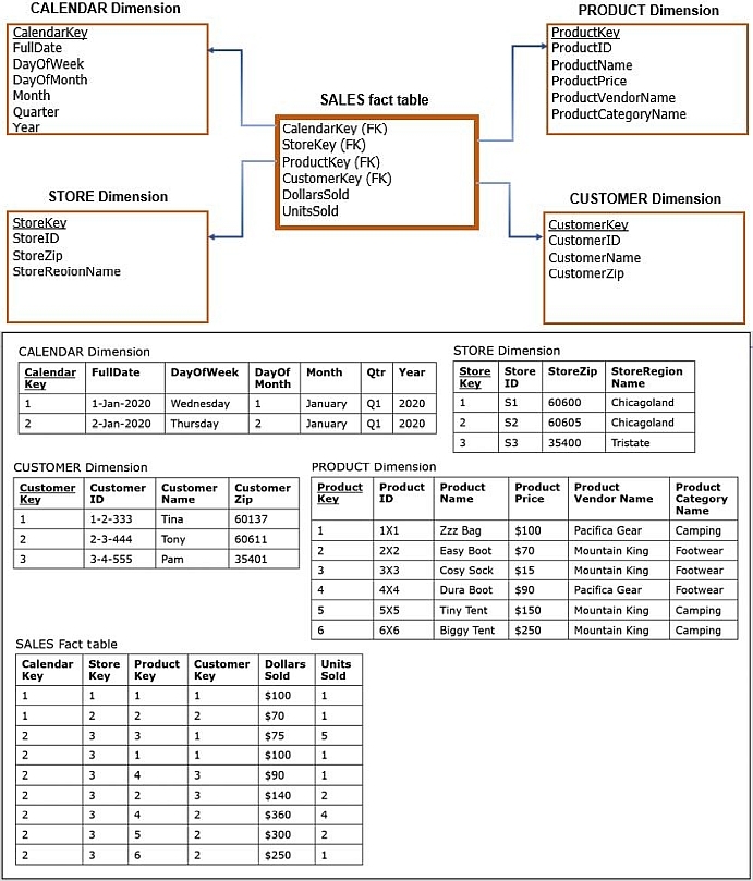
In the star schema, the chosen subject of analysis is represented by a fact table.
- In this example, the chosen subject of analysis (sales) is represented by the SALES fact table.
- The lower portion of the figure shows the populated tables of the star schema shown above.
- All of the data shown in each table was sourced from the data in the operational database source.
- Each record in the SALES fact table represents purchases of a particular product by a particular customer in a particular store on a particular day.
Designing the star schema involves considering which dimensions to use with the fact table that represents the chosen subject.
-
For every dimension under consideration, two questions must be answered:
- Question 1: Can the dimension table be created based on the existing data sources?
- Question 2: Can the dimension table be useful for the analysis of the chosen subject?
- In this particular example, there is only one available data source.
- The star schema in the figure above contains four dimensions: PRODUCT, STORE, CUSTOMER, and CALENDAR, and for each of these dimensions, the answer to both Question 1 and Question 2 was yes.
In the example above, a dimensional model was developed to analyze sales per product, customer, store, and date.
- Question 1 analysis confirms that for each of the dimensions under consideration, the existing operational database can provide the data source.
- Question 2 analysis confirms that each of the dimensions under consideration is useful.
-
Therefore, the team decided to create all four dimensions under consideration: PRODUCT, CUSTOMER, STORE, and CALENDAR.
-
Dimension PRODUCT is the result of joining table PRODUCT with tables VENDOR and CATEGORY from the
operational database, in order to include the vendor name and category name.
- It enables the analysis of sales across individual products as well as across products' vendors and categories.
- Dimension CUSTOMER is equivalent to the table CUSTOMER from the operational database.
- It enables the analysis of sales across individual customers as well as across customers' zip codes.
- Dimension STORE is the result of joining table STORE with table REGION from the operational database, in order to include the region name.
- It enables the analysis of sales across individual stores as well as across store regions and zip codes.
- Dimension CALENDAR captures the range of the dates found in the TDate (date of sale) column in the SALESTRANSACTION table in the operational database.
- Date-related analysis is one of the most common types of subject analysis.
- For example, analyzing sales across months or quarters is a common date-related analysis.
- Virtually every star schema includes a dimension containing date-related information.
- In this example, dimension CALENDAR fulfills that role because the structure of the CALENDAR dimension is expanded by breaking down the fill date into individual components corresponding to various calendar-related attributes (such as quarter, month, year, and day of the week) that can be useful for analysis.
-
Dimension PRODUCT is the result of joining table PRODUCT with tables VENDOR and CATEGORY from the
operational database, in order to include the vendor name and category name.
The dimensionally modeled database shown above makes it possible to easily create analytical queries, such as:
- Query A: Compare the quantities of sold products on Saturdays in the category Camping provided by the vendor Pacifica Gear within the Tristate region between the first and second quarter of the year 2020.
Such queries in dimensionally modeled databases can be issued by using SQL or by using Online Analytical Processing/Business Intelligence (OLAP/BI) tools.
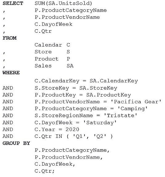
The following query uses the dimensional model to address Query A. This dimensional version will be referred to as Query A1.
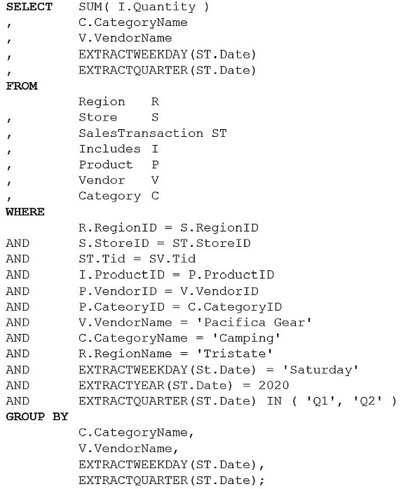
Using using the original nondimensional database makes queries more complex. Here is the nondimensional version (Query A2), which not only had to join more tables, but also requires user-defined functions to extract the year, quarter, and day of the week from the date.
Compare the two queries to observe the simplicity advantage for the analyst issuing a query on the dimensional model.
- Note that Query A1 (dimensional version) joins the fact table with three of its dimensions, while Query A2 (nondimensional version) joins seven tables and must use functions to extract the year, quarter, and day of the week from the date.
- This small example illustrates that, even in a simple case when the dimensional model is based on a small single source, analytical queries on the dimensionally modeled database can be significantly simpler to create than on the equivalent nondimensional database
The convenience of analysis with the dimensionally modeled data is even more evident in cases when data necessary for analysis resides in multiple sources, as discussed in Section 8.
- Situations when analytically useful data is located in multiple separate data systems and stores within an organization are very common.
Section 7: Characteristics of Dimensions and Facts
- A typical dimension contains relatively static data, while in a typical fact table records are added continually, and the table rapidly grows in size.
- In a typical dimensional database, dimension tables have orders of magnitude fewer records than fact tables.
Surrogate key
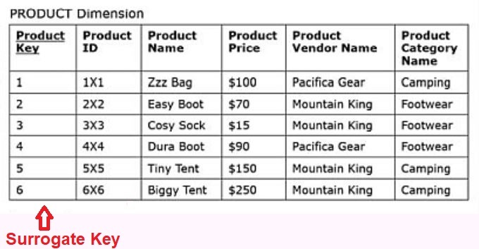
Often, dimension tables in a star schema will include a simple, non-composite system-generated key, also called a surrogate key.
- For example, instead of using the primary key ProductID as the primary key of the PRODUCT dimension, a new surrogate key column ProductKey is created.
- One of the main reasons for creating a surrogate primary key and not using the operational primary key as a primary key of the dimension, is to enable the handling of so called slowly changing dimensions (covered later).
- Values for the surrogate keys are typically simple auto-increment integer values.
- Surrogate key values have no meaning or purpose except to give each dimension a new column that serves as a primary key within the dimensional model instead of the operational key.
Section 8: Expanded Example: Dimensional Model Based on Multiple Sources
More commonly, data warehouses draw data from multiple sources.
The preceding dimensional modeling example depicts a scenario where an analytical database is based on a single source.
The following expansion of the initial example adds two additional data sources:
-
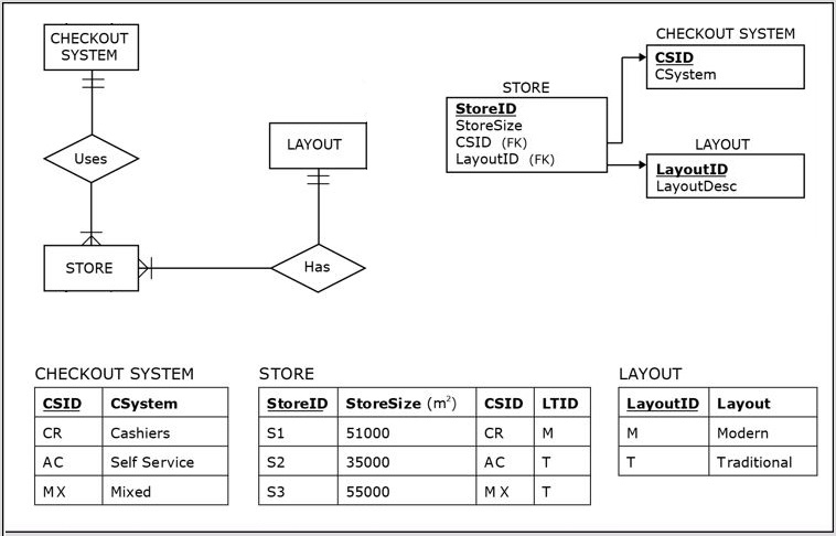
In addition to the Sales Department database, the facilities department maintains a database that contains the following information about the physical details of each of the individual stores: Store Size, Store Layout, and Store Checkout System. The Facilities Department database is shown below.
-
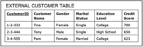
The company does not maintain demographic-related data of its customers in any of its operational databases, so they acquired the demographic-related data table for its customers from a market research company. This acquired external data source Customer Demographic data table is shown below.
The following figure shows an expanded dimensional model that is now based on three different data sources:
- two internal operational databases – the Sales Department database and the Facilities Department database
- and one external source – the Customer Demographic data table
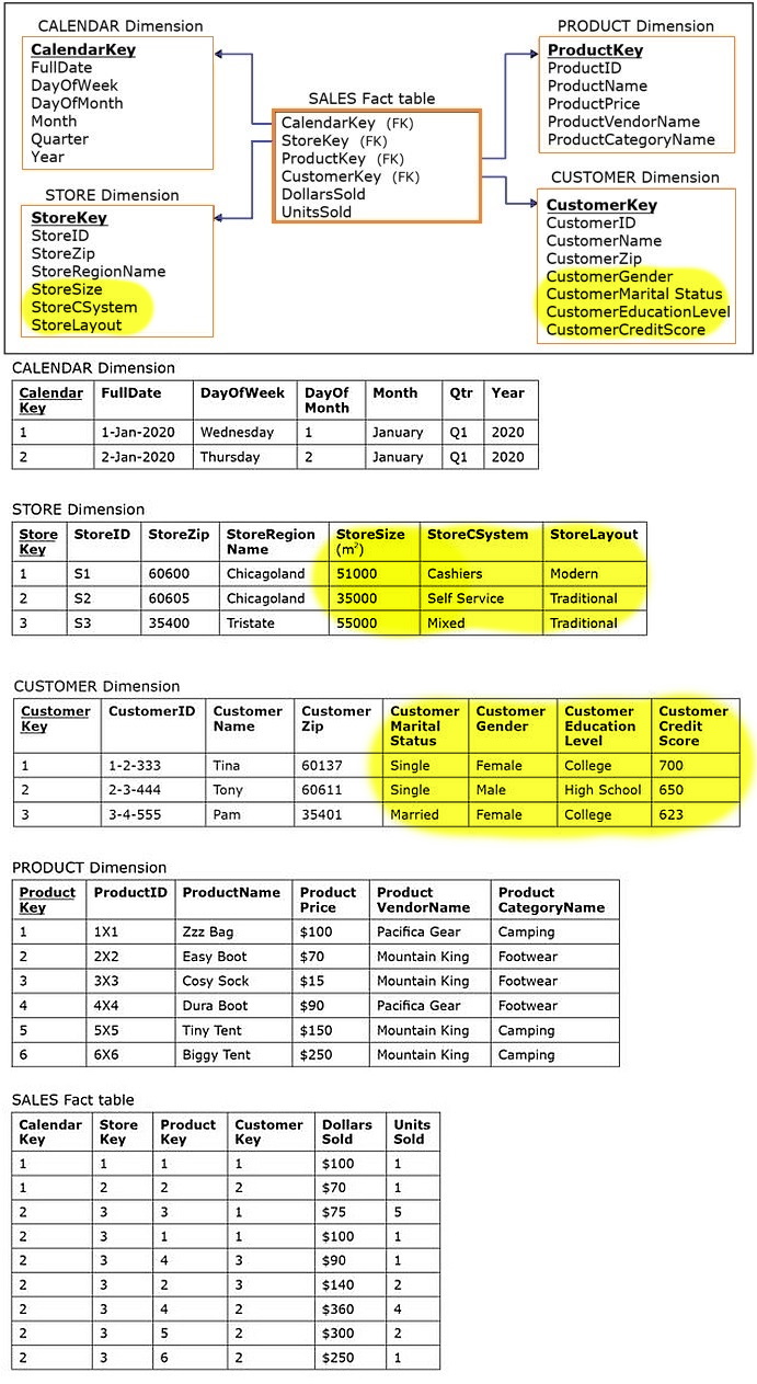
- Note that the data source Facilities Department database enabled the addition of columns StoreSize, StoreCSystem, and StoreLayout to the dimension STORE.
- Also note that the external data source Customer Demographic data table enabled the addition of columns CustomerGender, CustomerMaritalStatus, CustomerEducationLevel, and CustomerCreditScore to the dimension CUSTOMER.
The expanded model makes it possible to ask even more refined analytical questions that consider a larger variety of analysis factors. For example, consider the following question.
- Query B: Compare the quantities of sold products to male customers in Modern stores on Saturdays in the category Camping provided by the vendor Pacifica Gear within the Tristate region between the first and second quarter of the year 2020.
To obtain the answer to the Query B from the operational sources, a user would have to issue several queries spanning all three operational sources and then combine the results of those queries to receive the final answer.
Obtaining the answer to Query B using the dimensionally modeled database shown above is much more straightforward.
- Query B - dimensional version involves a simple extension of Query A1 (dimensional version):
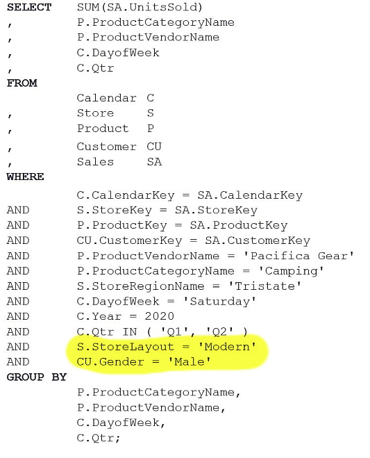
A query using dimensionally modeled data such as Query B above, could be created in an even simpler fashion by utilizing OLAP/BI tools.
Section 9: Additional Possible Fact Attributes
As mentioned earlier, a fact table contains
- foreign keys connecting it to the dimension tables and
-
the measures related to the subject of analysis.
- For example, if the subject of the business analysis is sales, typical measures in the fact table sales are the sales dollar amount and quantity.
In addition to the measures related to the subject of analysis, in certain cases fact tables can contain other attributes that are not measures, as illustrated by the following figure.
- A row in the SUBJECT fact table (named possible other FactAttributes) indicates that the fact table can contain other possible attributes that are not measures.
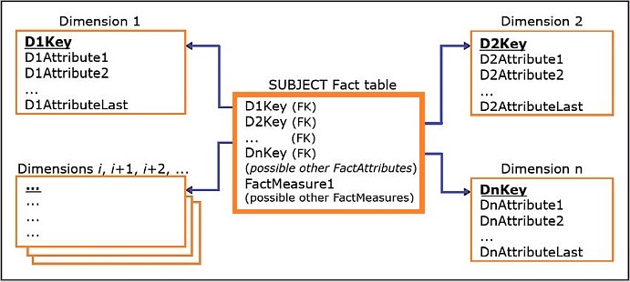
Two of the most typical additional attributes that can appear in the fact table are
- the transaction identifier and
- the transaction time
These two additional attributes will be discussed next.
Transaction Identifier in the Fact Table
First, the transaction identifier concept is demonstrated.
-
In the Sales Department Database shown in Section 2, the SALES TRANSACTION relation has a transaction identifier column TID.
- The TID values do not appear at first glance to have any analytical value.
-
However, for certain types of analysis, the TID values can provide additional insight.
- For example, in this case the TID value can provide information about which products were sold within the same individual transaction.
- Such information is useful for a variety of analytical tasks.
- One type of analysis that seeks to establish which products often sell together is commonly referred to as market basket analysis (also known as "association rule mining" or "affinity grouping") and including the TID in the dimensional model would allow business analysts to use this type of analysis.
-
Once the decision is made to include the TID in the dimensional model, the question remains: Where in the star schema should the TID appear?
-
At first glance, one option is to create a separate TRANSACTION dimension, which would include the TID attribute.
- However, as we mentioned earlier, in a typical properly designed star schema, the number of records (rows) in any of the dimension tables is relatively small when compared to the number of records (rows) in the fact table.
- If we create a separate TRANSACTION dimension, the number of records in that dimension would be at the same order of magnitude (e.g., millions or billions of records) as the number of records in the SALES fact table and, at the same time, at orders of magnitude higher than the number of records in any other dimension.
-
At first glance, one option is to create a separate TRANSACTION dimension, which would include the TID attribute.
-
A more practical approach is to include the TID as an additional column in the fact table, as shown below:
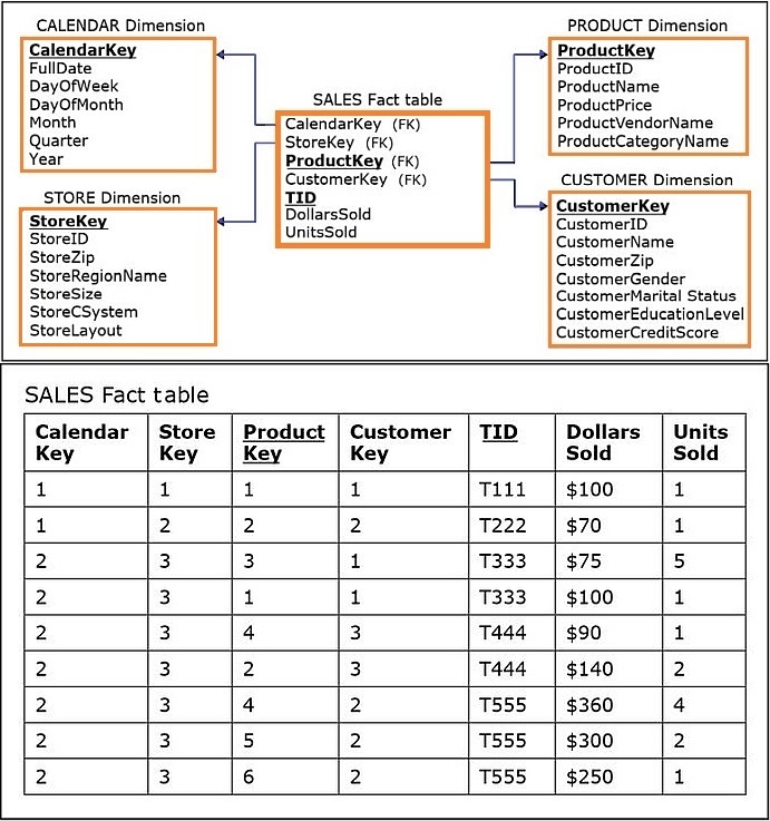
- This simple approach still enables the analysis that considers which products were sold within the same transaction, without the need for creating an additional dimension that would contain an enormous number of records.
- In practice, the transaction identifier can be represented as sales transaction identifier, order identifier, rental identifier, ticket identifier, bill identifier, and so on.
-
The approach of including a transaction identifier in the fact table is often referred to in the literature and practice as a degenerate dimension, where the term "degenerate" signifies "mathematically simpler than."
- The term merely indicates that it is simpler to include an event identifier within the fact table than to create a separate dimension for it.
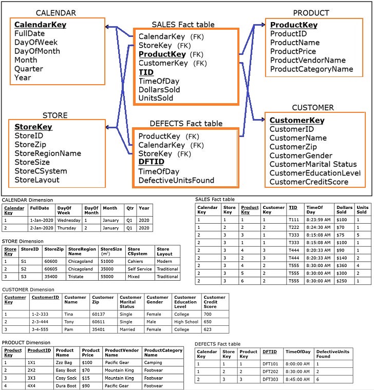
- The lower portion of the above figure shows the records in the SALES fact table in the dimensional model for the subject sales, populated with the data, including the transaction identifier (TID) values in each row.
In the SALES fact table for the dimensional model shown above, the primary key is comprised of the TID and ProductKey columns, because each record in the fact table refers to a particular line item of a particular sale transaction.
- TID is not unique in the table because more than one product can be bought in the same transaction.
- Similarly, ProductKey is not unique because the same product can be associated with more than one transaction
- Hence, both TID and ProductKey are needed to form the composite primary key.
- Note that all foreign keys referring to the dimensions are mandatory in the fact table (i.e., none of the foreign keys are optional).
- Each record in the fact table must refer to one record in each of the dimensions that the fact table is connected to.
Transaction Time in the Fact Table
In order to examine the transaction time concept, let us assume that the business analysts analyzing subject sales would like to incorporate the time of day into their analysis.
- The previous example can be slightly expanded by adding the transaction time (TTime) attribute to the SALESTRANSACTION entity and to the resulting SALESTRANSACTION relation.
-
The following figure shows the SALESTRANSACTION table populated with the data, demonstrating the changing time of day values in column TTime, while all other columns in the SALESTRANSACTION table remain unchanged.
-
In order to reflect time of day information in the dimensional model, time can be added as another attribute to the fact table, as shown below, making any type of time-of-day-related business analysis possible.
- Note that the concept of including a transaction identifier column and a time of day column in the fact table is applicable to any scenario in which event transactions, such as purchase transactions, orders, rentals, tickets, and bills, provide a basis for a fact table.
Section 10: Multiple Fact Tables in a Dimensional Model
A dimensional model can contain more than one fact table, a situation that occurs when multiple subjects of analysis share dimensions.
A dimensional model with multiple fact tables is referred to as a constellation (galaxy) of stars.
- This approach allows for quicker development of analytical databases for multiple subjects of analysis, because dimensions are reused instead of duplicated.
- Further, due to the sharing of dimensions, this approach enables straightforward cross-fact analysis, such as a comparison of the average daily number of products sold vs. the average daily number of defective products found and removed per store, region, quarter, product category, and so on.
In the following scenario, in addition to the tracking of sales by the sales department, the quality control department tracks occurrences of defective products in its stores.
- The quality control department regularly inspects the shelves in all of the stores, and when a defective product is found, it is removed from the shelf.
- For each instance of a found-and-removed defective product, the quality control department staff member immediately records the time, date, defect type, and product information in the Quality Control Department database.
-
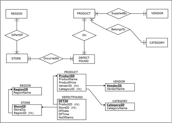
The ER diagram and the resulting relational schema of the Quality Control Department database is shown in the following figure.
- slowly
The next figure shows the records in the Quality Control Department database, whose ER diagram and relational schema are shown above
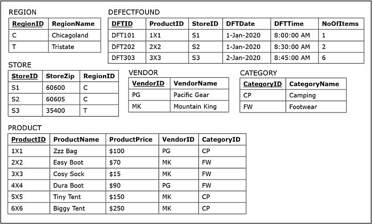
- Some of the information in the Quality Control Department database overlaps with the information in the Sales Department database, such as information about the stores and products being included in both databases.
- It is very common for organizations to have separate operational databases with overlapping information.
The goal is to analyze the defects in the same manner as sales, so a dimensional model will be created in order to analyze the occurrences of defective products found in stores.
- The dimensions that are needed to analyze defects are already created for the dimensional model for the analysis of sales.
-
Hence, another fact table for defects can be created as a part of the already existing dimensional model, as opposed to creating a separate new dimensional model, as shown below.
Section 11: Detailed Versus Aggregated Fact Tables
Fact tables in a dimensional model can contain either detailed data or aggregated data.
- In detailed fact tables each record refers to a single fact.
- In aggregated fact tables each record summarizes multiple facts.
The following example illustrates the difference between the two types of data in fact tables.
-
To explain these concepts, the set of data in the Sales Department operational database will be slightly expanded by adding one more record in the SALESTRANSACTION table and two more records in the INCLUDES table, as shown below.
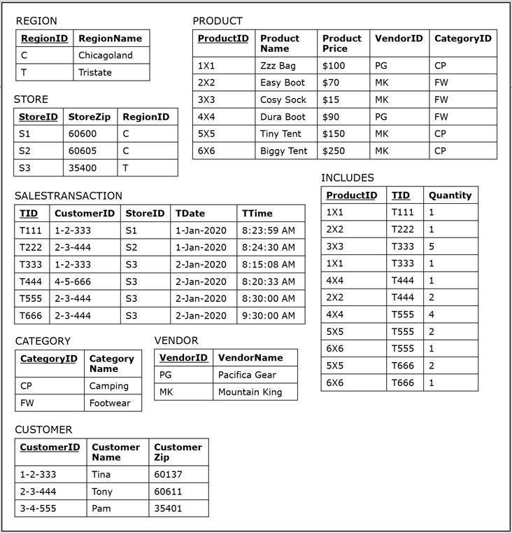
- In this expanded scenario, customer Tony, who had already bought two Tiny Tents and one Biggy Tent in store 53 at 8:30:00 AM, came back to the same store and made the identical purchase one hour later at 9:30:00 AM because, well, you can never have too many tents.
- This slight expansion of the data set will help us to better illustrate the difference between detailed and aggregated star schemas in the examples below.
Detailed Fact Table
-
The figure below shows the SALES fact table from the dimensional model in Section 8 populated with data, where additional records are added to the SALES fact table based on the additional records in the figure above.
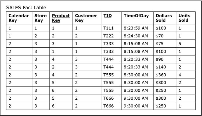
- Because the SALES fact table above is detailed, each record in it refers to one sales fact represented by one record in the INCLUDES table in the figure of the Sales Department operational database at the top of this section.
- Hence, both the SALES and INCLUDES tables have 11 rows.
Aggregated Fact Table
-
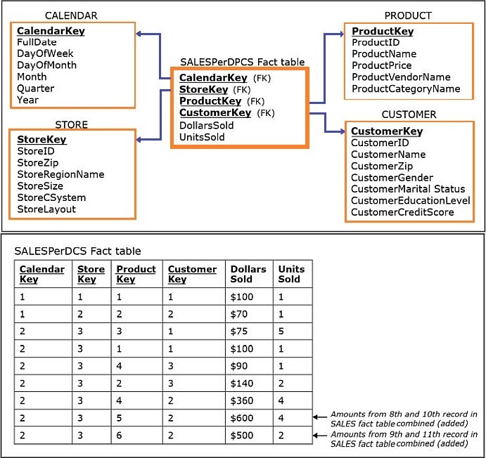
In contrast, the next figure shows a dimensional model containing an aggregated fact table (SalesPerDPCS – per day, product, customer, and store) for the subject sales.
-
The primary key of this aggregated fact table is composed of the CalendarKey, StoreKey, ProductKey, and CustomerKey columns.
- Each record in the SALES fact table refers to a summary representing the amount sold in dollars and units on a particular day for a particular product for a particular customer in a particular store.
- The SalesPerDPCS table in the figure above has only nine records because it is an aggregated fact table.
-
In particular:
- The 8th record in the aggregated SalesPerDPCS fact table above summarizes (adds together) the 8th and 10th records from the detailed SALES fact table, and, consequently the 8th and 10th records from the INCLUDES table in the above figure showing data records for the Sales Department Database.
- The 9th record in the aggregated SalesPerDPCS fact table above summarizes the 9th and 11th records from the detailed SALES fact table and, consequently, the 9th and 11th records from the INCLUDES table in the above figure showing data records for the Sales Department Database.
-
The aggregation occurs because the TID values are not included in the aggregated SalesPerDPCS fact table in the above figure.
- The first seven records in the aggregated SalesPerDPCS fact table shown above are summarizations of a single sales fact.
- Therefore, their values are equivalent to the values in the first seven records in the SALES fact table in detailed SALES fact table, as well as to the values in the first seven records in the INCLUDES table in the above figure showing data records for the Sales Department Database.
- This is because in those seven cases there was only one sale of a particular product to a particular customer in a particular store on a particular day.
- The 8th and 10th records and the 9th and 11th records originate from two transactions in which the same two products were purchased by the same customer in the same store on the same day.
-
The primary key of this aggregated fact table is composed of the CalendarKey, StoreKey, ProductKey, and CustomerKey columns.
The example above is one of the many ways in which the data from the source in the above figure showing data records for the Sales Department Database could have been aggregated.
Another example of a dimensional model with an aggregated sales fact table (SalesPerDCS – per day, customer, and store) is shown in the following figure.
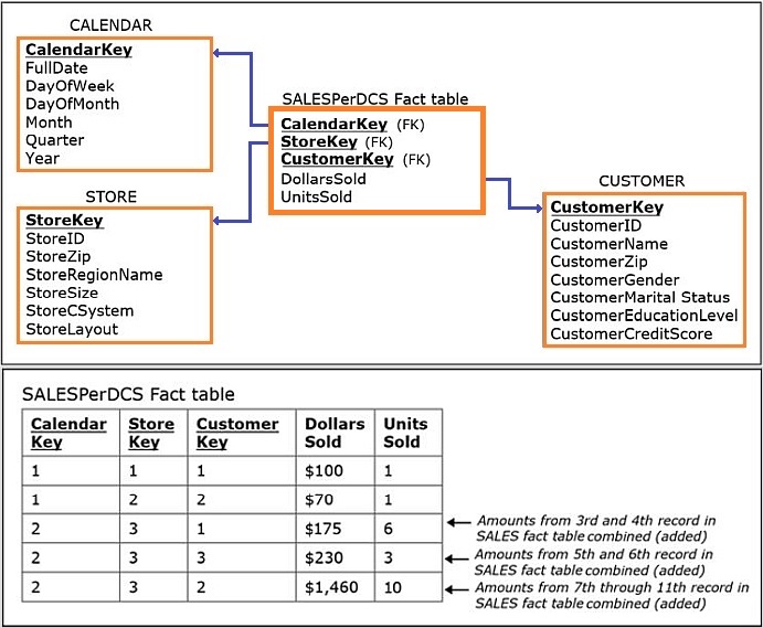
- The upper part of the figure shows a dimensional model that aggregates the same data as the dimensional model in the aggregated sales fact table (SalesperDPCS), but in a different (coarser) fashion.
- The upper part of the figure shows the aggregated fact table in the dimensional model from the aggregated sales fact table (SalesperDCS) populated with data.
- In the figure above, the primary key of the aggregated fact table SALES is comprised of the CalendarKey, StoreKey, and CustomerKey columns.
- The ProductKey is not included as a column in the table SALES, because the table contains an aggregation of data over all products.
- Each record in the aggregated fact table SALES refers to a summary representing the quantities in dollars and units of all products bought on a particular day in a particular store by a particular customer.
-
The aggregated fact table SalesPerDCS in the figure above has five records, and the bottom three records contain the following summarizations:
- The 3rd record in SalesPerDCS summarizes the 3rd and 4th records from the SALES fact table in the detailed SALES fact table, and, consequently the 3rd and 4th records from the INCLUDES table in the figure showing data records for the Sales Department Database.
- The 4th record in SalesPerDCS summarizes the 5th and 6th records from the SALES fact table in the detailed SALES fact table, and, consequently, the 5th and 6th records from the INCLUDES table in the figure showing data records for the Sales Department Database.
- The 5th record in SalesPerDCS summarizes the 7th through 11th records from the SALES fact table in the detailed SALES fact table, and, consequently, the 7th through 11th records from the INCLUDES table in the figure showing data records for the Sales Department Database.
-
The first two records in the aggregated SalesPerDCS fact table in the figure above are summarizations of a single sales fact, and therefore the values are equivalent to the values in the first two records in the SALES fact table in the detailed SALES fact table, as well as to the values in the first two records in the INCLUDES table in the figure showing data records for the Sales Department Database.
- This is because those two records represent instances when there was only one product bought by a particular customer in a particular store on a particular day.
- When more than one product was bought by a customer in a particular store on a particular day, the records are aggregated in the SalesPerDCS fact table in the figure above.
Section 12: Granularity of the Fact Table
The granularity of the table describes what is depicted by one row in the table.
- Detailed fact tables have fine level of granularity because each record represents a single fact.
- Aggregated fact tables have a coarser level of granularity than detailed fact tables as records in aggregated fact tables always represent summarizations of multiple facts.
Here are some examples:
- The SalesPerDPCS fact table in the aggregated sales fact table (SalesperDPCS) has a coarser level of granularity than the SALES fact tables in the detailed SALES fact table because, as we have shown, records in the SalesPerDPCS fact table summarize records from the SALES fact table in the detailed SALES fact table.
- The SalesPerDCS fact table in the aggregated sales fact table (SalesperDCS) has an even coarser level of granularity, because its records summarize records from the SalesPerDPCS fact tables in the aggregated sales fact table (SalesperDPCS).
- The 3rd record in the SalesPerDCS summarizes the 3rd and 4th records from the SALES fact table in the detailed SALES fact table and also summarizes the 3rd and 4th records from the SalesPerDPCS fact tables in the aggregated sales fact table (SalesperDPCS).
Granularity of the fact tables
- Due to their compactness, coarser granularity aggregated fact tables are quicker to query than detailed fact tables.
- Coarser granularity tables are limited in terms of what information can be retrieved from them.
- Aggregation is requirement-specific, while a detailed granularity provides unlimited possibility for analysis, therefore, you can always obtain an aggregation from the finest grain but the reverse is not true.
-
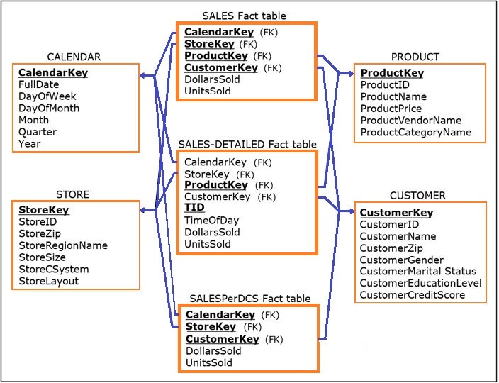
One way to take advantage of the query performance improvement provided by aggregated fact tables, while retaining the power of analysis of detailed fact tables, is to have both types of tables coexisting within the same dimensional model, i.e. in the same constellation, as in the figure below.
Line-Item Versus Transaction-Level Detailed Fact Table
Detailed fact tables can represent different types of information, depending on what is depicted by the underlying data sources.
The two most common types of detailed fact tables are line-item fact tables and transaction-level fact tables.
- Line-item detailed fact table – Each row represents a line item of a particular transaction.
- Transaction-level detailed fact table – Each row represents a particular transaction.
Section 13: Slowly Changing Dimensions and Timestamps
A typical dimension in a star schema contains either
- Attributes whose values do not change (or change extremely rarely) such as store size and customer gender.
- Attributes whose values change occasionally and sporadically over time, such as customer zip and employee salary.
A dimension that contains attributes whose values can change is often referred to as a slowly changing dimension.
There are several different approaches to dealing with slowly changing dimensions, with the most common referred to as Type 1, Type 2, and Type 3.
-
Type 1 Approach
- Changes the value in the dimension’s record, where the new value replaces the old value.
- No history is preserved.
- The simplest approach, used most often when a change in a dimension is the result of an error.
-
Type 2 Approach
- Creates a new additional dimension record using a new value for the surrogate key every time a value in a dimension record changes.
- Used in cases where history should be preserved.
-
Can be combined with the use of timestamps and row indicators.
- Timestamps – columns that indicates the time interval for which the values in the records are applicable.
- Row indicator – column that provides a quick indicator of whether the record is currently valid.
-
Type 3 Approach
- Involves creating a "previous" and "current" column in the dimension table for each column where changes are anticipated.
- Applicable in cases in which there is a fixed number of changes possible per column of a dimension, or in cases when only a limited history is recorded.
- Can be combined with the use of timestamps.
- Some sources list up to six types.
Section 14: Comparing ER Modeling and Dimensional Modeling as Data Warehouse Design Techniques
ER modeling
ER modeling is a technique for facilitating the requirements collection process, where all requirements are collected and visualized as the ER model constructs: entities, attributes, and relationships.
- The ER model provides a clear visualization of the requirements (i.e., conceptual model) for the data warehouse that is to be created.
- The ER model of a data warehouse is subsequently mapped into a relational schema, which is then implemented as a normalized database that hosts the data warehouse.
Dimensional modeling
Dimensional modeling can be used both for visualizing requirements for a data warehouse (i.e., conceptual modeling), and for creating a data warehouse model that will be implemented (i.e., logical modeling).
- When dimensional modeling is used to facilitate the data warehouse requirements collection process, then the requirements collection involves determining which subjects will be represented as fact tables, and which dimensions and dimension attributes will be used to analyze the chosen subjects.
- Once the requirements are represented as a dimensional model, the dimensional model can also be directly implemented in a DBMS as the schema for the functioning data warehouse.
Making a Choice
Both ER modeling and dimensional modeling are viable alternatives for modeling data warehouses/data marts, and can be used within the same project.
Using one technique for visualizing requirements does not preclude using the other technique for creating the model that will actually be implemented.
- Dimensional modeling might be used during the requirements collection process for collecting, refining, and visualizing initial requirements.
- Based on the resulting requirements visualized as a collection of facts and dimensions, an ER model for a normalized physical data warehouse can be created if there is a preference for a normalized data warehouse.
- Once a normalized data warehouse is created, a series of dependent data marts can be created using dimensional modeling.